How to control line spacing in blogger

This is a very short post, I have been using a very interesting plugin for inserting code, and the a variety of languages are impressing. This is Pygments for Windows Live Writer.
To my surprise I discovered the rather annoying (Enter –> double line spacing conversion) which is really an annoying convention adopted by blogger and for the new editor (what they call new look) the old setting –> Formatting –> No line breaks is absent.
What I found that could solve this problem. Go to posts from the browser and pick any old post and choose options on the right hand side and choose the radio button Enter to line Breaks. That should eliminate all the extra spaces in the inserted code.
As to whether it will be systematically applied to all the future posts I am not sure of it. But I kind of hope that it will persist, because it is really cumbersome to edit every post in the browser after posting it from the Windows Live Writer.

As a way to test if it will have double spacing or not? I have tried it and it does not work. Every time I will insert a code I have to edit it from the Browser.

Python vs. Matlab

I was familiar with Python as an introduction language fro programming, I tried a couple of time a long time ago. The main impression that I had was that it is a bit slow although it still quite reasonable choice for prototyping specially it is free and platform independent.

I thought to revisit my old interest in Python, and here is an implementation of Julia sets that I fetched from a lecture on YouTube, one of many available that was delivered at scipy conferences. The problem is that I connot remember which one now that I watched.

import numpy as np
from time import time

def kernel(z, c, lim, cutoff=1e6):
    ''' Computes the number, `n`, of iterations necessary such that
    |z_n| > `lim`, where `z_n = z_{n-1}**2 + c`.
    '''
    count = 0
    while abs(z) < lim and count < cutoff:
        z = z * z + c
        count += 1
    return count

def compute_julia(c, N, bound=2, lim=1000., kernel=kernel):
    ''' Pure Python calculation of the Julia set for a given `c`.  
    No NumPy array operations are used.
    '''

    julia = np.empty((N, N), dtype=np.uint32)
    grid_x = np.linspace(-bound, bound, N)
    grid_y = grid_x * 1j
    c = complex(c)
    t0 = time()
    for i, x in enumerate(grid_x):
        for j, y in enumerate(grid_y):
            julia[i,j] = kernel(x+y, c, lim)
    return julia, time() - t0

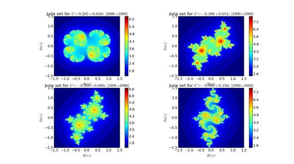
This two functions composed of the iterative kernel and the actual computation of the Julia set values on a grid composed of \(N X N \) grid.
The plotting part are as given below

import pylab as pl
def plot_julia(kwargs, compute_julia):
    ''' Given parameters dict in `kwargs` and a function to                    compute the Julia set (`compute_julia`), plots the 
       resulting Julia set with appropriately labeled axes.
    '''
    kwargs = kwargs.copy()
    def _plotter(kwargs):
        bound = kwargs['bound']
        julia, time = compute_julia(**kwargs)
        print "execution time (s):", time
        julia = np.log(julia)
        pl.imshow(julia,
                  interpolation='nearest',
                  extent=(-bound, bound)*2)
        pl.colorbar()
        title = r"Julia set for $C={0.real:5.3f}+{0.imag:5.3f}i$ $[{1}\times{1}]$"
        pl.title(title.format(kwargs['c'], kwargs['N']))
        pl.xlabel("$Re(z)$")
        pl.ylabel("$Im(z)$")
    pl.figure(figsize=(14, 12))

    cvals = [0.285+0.01j, -0.1+0.651j, -0.4+0.6j, -0.8+0.156j]
    subplots = ['221',    '222',       '223',     '224'      ]

    for c, sp in zip(cvals, subplots):
        kwargs.update(c=c)
        pl.subplot(sp)
        _plotter(kwargs)
    pl.show()

And here is the implementation

kwargs = dict(N=1000, bound=1.5)
plot_julia(kwargs, compute_julia)

and here is the output on my machine,

The execution times for the four figures was

execution time (s): 37.7200000286
execution time (s): 97.0900001526
execution time (s): 44.8949999809
execution time (s): 72.1289999485

Somewhat slow !! 

The matlab implementation of the same function are shorter and considerably faster.

function julia = compute_julia(N, bound, c)

    julia = uint32(zeros(N, N));
    grid_x = linspace(-bound, bound, N);
    grid_y = grid_x * 1j;

    for j  = 1:N
        for i  = 1:N
            julia(i,j) = kernel(grid_x(i)+grid_y(j), c);
        end
    end
end

function count = kernel(z, c)

    %Computes the number, `n`, of iterations necessary such that
    %|z_n| > `lim`, where `z_n = z_{n-1}**2 + c`.

    lim=1000;
    count = 0;
    cutoff=1e6;
    while abs(z) < lim && count < cutoff
        z = z * z + c;
        count = count + 1;
    end
end

And now for the actual computation with the same values as the ones used in the python code

cvals = [0.285+0.01j, -0.1+0.651j, -0.4+0.6j, -0.8+0.156j];
for i = 1:4
    tic; julia = compute_julia(1000, 1.5, cvals(i)); toc
    subplot(2,2,i)
    image(julia)
end

and here are the execution times

Elapsed time is 7.515207 seconds.
Elapsed time is 20.076634 seconds.
Elapsed time is 8.709530 seconds.
Elapsed time is 14.150072 seconds.

So, clearly the matlab is faster. But what if we used Cython with python and mex files with matlab? The cython implementation is really one of the best automatic code generation tools ever. The ease with which the conversion is done is unsurpassed.

First and since I am using the Ipython –notebook we have to load the Cython magic

%load_ext cythonmagic

%%cython

from time import time
import numpy as np
cimport cython
cimport numpy as cnp
ctypedef double complex cpx_t
ctypedef double         real_t

cdef inline real_t cabs_sq(cpx_t z) nogil:
    ''' Helper inline function, computes the square of the abs. 
        value of the complex number `z`.
    '''
    return z.real * z.real + z.imag * z.imag

cpdef unsigned int kernel(cpx_t z,
                          cpx_t c,
                          real_t lim,
                          real_t cutoff=1e6) nogil:
    ''' Cython implementation of the kernel computation.
        This is implemented so that no
        C-API calls are made inside the function
        body.  Even still, there is some overhead as compared 
        with a pure C implementation.
    '''
    cdef unsigned int count = 0
    cdef real_t lim_sq = lim * lim
    while cabs_sq(z) < lim_sq and count < cutoff:
        z = z * z + c
        count += 1
    return count

@cython.boundscheck(False)
@cython.wraparound(False)

def compute_julia_opt(cpx_t c,
                       unsigned int N,
                       real_t bound=1.5,
                       real_t lim=1000.):
    '''
    Cython `compute_julia()` implementation with Numpy array buffer
    declarations and appropriate compiler directives.  The body of this
    function is nearly identical to the `compute_julia_no_opt()` 
    function.
    '''
    cdef cnp.ndarray[cnp.uint32_t, ndim=2, mode='c'] julia
    cdef cnp.ndarray[real_t, ndim=1, mode='c'] grid
    cdef unsigned int i, j
    cdef real_t x, y

    julia = np.empty((N, N), dtype=np.uint32)
    grid = np.linspace(-bound, bound, N)
    t0 = time()
    for i in range(N):
        x = grid[i]
        for j in range(N):
            y = grid[j]
            julia[i,j] = kernel(x+y*1j, c, lim)
    return julia, time() - t0

This only an alternative implementation of the of the compute Julia sets. No modification is made to the plotting function. The results of the execution time is !!!

execution time (s): 0.107000112534
execution time (s): 0.279000043869
execution time (s): 0.123000144958
execution time (s): 0.197000026703

Well that was fast, I used anaconda python distribution, with the MinGW package within it to compile the code with the accelerate module activated. 

Now for the comparison to be fair we need to use a similar acceleration trick, by transforming the matlab code into a mex file. This is done and the comparison of the execution times used by matlab mex function with VS 2012 as compiler is given below

Elapsed time is  0.828125000000000 seconds
Elapsed time is  2.140625000000000 seconds
Elapsed time is  0.953125000000000 seconds
Elapsed time is  1.484375000000000 seconds

So even when loading the mex file Cython is faster than matlab, and considering that I am still novice in both the mex files and python –cython conversions. I am sure there is still a huge room for improvement. But this is pretty impressive work by the python and cython community . I am considering seriously migrating completely to Python. 

Blasius Equation: Some Explorations Part 4

Boundary Layer Thickness

There is no sharp outer edge of the boundary layer. Rather it merges smoothly and gradually with the outer free stream. However, there are several rational ways of defining a boundary layer thickness, and we consider one of them here. The idea is determining where the horizontal velocity is nearly equal to the free stream velocity or a constant ratio of it. The thickness , is the y-value at which the u velocity is 0.90 of the free stream velocity. In order to find that value we have need to wrap the previous pieces of code into a single function which is listed below

---

function [eta, fun] = BLThickness(x, lim)
    function B= BlasVal(y)
        options = odeset('RelTol', 1e-10, 'AbsTol', 1e-12);
        sol=ode45(@BlasiusFunc, [0,15], [0.0 0.0 1.0], options);
        alpha = sqrt(sol.y(2,end));
        f = (deval(sol, (y./alpha)));
        B = (f(2)./alpha^2)-lim;
       
        function df = BlasiusFunc(~,f)
            df = zeros(3,1);
            df(1) = f(2);
            df(2) = f(3);
            df(3) = -f(1)*f(3)/2;
        end
    end

    [eta, fun]= fzero(@BlasVal, x);
end

---

So, in order to compute the value of the \(\eta_{90}\)

BLThickness(3, 0.9)

This gives the value of that corresponds to \(\frac{u}{U_{\infty}}\)=0.90. So the thickness of the boundary layer is given by: \[\delta_{90} = \eta_{90} \delta = \eta_{90} \sqrt{\frac{\mu x}{U_{\infty}}} \]